I have a fair number of HO model train “cab ride” videos on my YouTube channel. I particularly enjoy a view where the camera follows the last car, or precedes the front engine. Over the years I’ve been experimenting with various ways to achieve them, and I’m currently using this setup where a camera car is attached to the HO model train using a 3d-printed long rod:

The camera car setup.

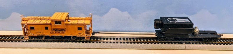
For further details, you can read this blog post that explains the camera car setup.

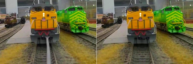
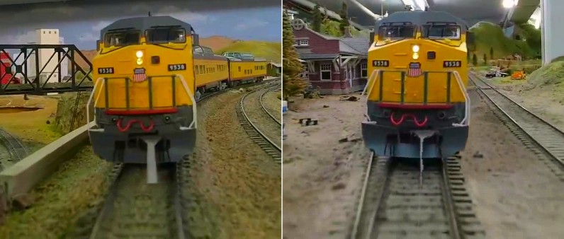
Back in 2023, I wrote a DaVinci Resolve plugin that “erases” the rod, which is very visible on camera and quite distracting:

Original image captured by camera               Desired image for the final video

However that plugin is a bit cumbersome to use. It’s basically a flood fill algorithm based on luma thresholds that need to be adjusted multiple times along a video -- in a typical video, I end up having to do keyframe editing on the plugin parameters almost every other frame. The plugin setup is a bit involved also as it first requires creating a DaVinci Fusion tracker to find the location of the coupler at the top of the rod. That process itself is finicky as we lose the tracker as soon as the train enters a tunnel.

The rod detection also leaves to be desired. Being written as a Fuse in Lua, I’m fairly limited on what I can use when performing the rod detection: the image is first converted from RGB to HLS, and we work on the Luminance channel, scanning the image vertically top to button below the coupler, and identifying the left and right contrast edges of the rod for each scan line. This fails when there’s not enough difference between the rod and the rails or the ballast. It also fails in tunnels or other areas with poor illumination. That’s why the contrast thresholds need to be adjusted fairly frequently over the frame sequence.

Recently I’ve been using numpy and OpenCV for another project at home, and that gave me some idea on how I could approach the rod detection algorithm differently.

The first difference is that we’d write a preprocessor: an external program processes the source video and creates a copy without the rod, and then we just use the result in DaVinci Resolve like a normal video. That will dramatically speed up edits and rendering in DaVinci as it no longer needs to apply the plugin every time the editor renders the video.

The immediate benefit is that we can now process the video using multiple passes. That’s actually a major limitation in the Fuse Lua plugin: it only processes a single frame at a time, without any other context. However here we have the advantage that the rod movement is relatively smooth along the video. If we find the rod’s location once, we can use that information to approximate its location for the next frames. We can also do something that the immediate-frame based approach of the plugin can never achieve: do a first pass on the entire video, skip frames of low quality where the rod detection does not work, and then later interpolate the rod location for all missing frames.

Properties

Let’s look at the original image captured by the camera:

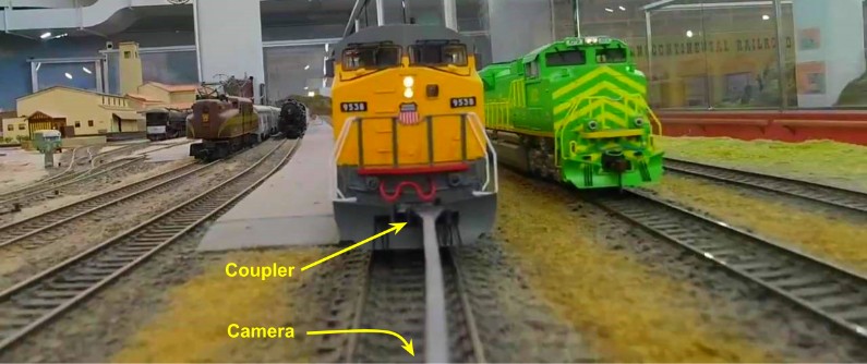
There are a few interesting properties which we should be able to take advantage of:

• The camera is, by definition, “centered”, so the bottom of the rod is always somewhere near the center of the screen.
• That however fluctuates in curves as the rod tends to pivot right or left. So we cannot assume it’s perfectly straight and vertical in the image. It may be slanted and slightly bent during curves, and definitely not centered anymore.
• Obviously the coupler is going to swing right and left during curves.
• The rod has a fixed length, and the perspective is mostly constant. That means the coupler is always more or less at the same height. It also fluctuates based on track geometry.
• The perspective is fixed. That means we can measure the width of the rod at the top and the bottom and these values are fairly constant.
• We capture the video at 30 fps, thus movements are relatively smooth from one frame to the next. There’s a lot of temporal consistency we can use. That’s the part we were missing in the DaVinci Fuse processing. Here we can have temporal filters that reject rod locations if they are drastically different from the ones from the previous frame.
• If we look at the image vertically, the rod is this vertical smooth gray area, whereas the track has ties which must form some kind of alternating contrast.
• As the train moves, the rod is mostly at the same location from one frame to the next, and so that smooth gray area is essentially the same between two consecutive frames. On the other hand, the track and its ties will move vertically as the train advances.

Overview of PyRod 1

The previous iteration was a DaVinci Fusion plugin: the workflow was to load the video in Resolve, apply the plugin as a Fusion node, and let the Fuse plugin remove the rod on the current frame, either in the Edit/Cut page, or when computing the final video. The new PyRod would work differently: we call a Python script that loads the video using OpenCV, processes it, and creates a new video without the rod. Then just load that video in Resolve as a normal one.

GitHub: https://github.com/alf-labs/rod/tree/main/pyrod1 

The structure of the Python project is as follows:

• setup.sh: A wrapper script to create a Python Virtual Environment and install the numpy and opencv-python packages. OpenCV can be quite tricky to install -- it comes with a number of prebuilts that are tightly linked to specific versions of Python depending on whether you run it on Linux or Windows MSYS. Trying to build from scratch is an exercise in frustration that rarely ends well.
• pyrod.py: the main entry point. It decodes command line parameters, loads the input video, invokes one or more “processors”, and writes the output video and json data.
• processor.py: the base class for processors. A processor performs one pass on the video, receiving all the video decoded frames. A processor returns the video to be output, and accumulates whatever data is needed for a later pass. The data can be saved and then reloaded as JSON.
• process_locator.py: the first pass processor. It locates the base of the rod in the image. Details below.
• process_detector.py: the second pass processor. It determines the outline of the rod and generates the inpainting that replaces the rod.

Locating the Base of the Rod

The main idea behind the first version of PyRod (a.k.a. PyRod 1) was to try to find the rod automatically in the image. One of the time-consuming tasks in the earlier DaVinci Fusion plugin was to place a tracker on the coupler to find its location across the entire video.

However, when we look at the raw source image posted above, we can see that the rod necessarily crosses the bottom of the image, somewhere near the center. What we want is to detect a vertical band that is fairly smooth, and should ideally contrast easily on a background that, by design, must not be smooth -- either ballast on the side of the rails, or ties between the rails.

And that’s where numpy is going to become useful, because suddenly I can easily compute a Coefficient of Variation: “The coefficient of variation (CV) is defined as the ratio of the standard deviation σ to the mean μ.”

So here’s what we do: we’re going to analyze each vertical column of N pixels at the bottom of the image, and compute the coefficient of variation for each column of pixels. That gives us a 0..1 number that indicates if this column is either smooth (likely the rod) or not smooth (likely the ties or the ballast). We get an horizontal array of these CV values, and we just need to identify the peak (or valley). Because we know the size of the rod (it’s fixed after all), we can easily filter out noise.

That’s what happens in the process_locator.py. Here’s the debug output of the processor:

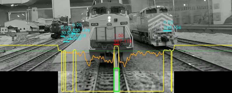
First, the image is converted from RGB to L*a*b, and we only use the luminance channel. Since we want to analyze contrast, the luminance is the best choice. We only analyze a limited region of interest at the bottom of the image -- 120 pixels high in this case, and about 50% of the image width.

Since it’s all about contrast, we can enhance contrast by applying a Contrast Limited Adaptive Histogram Equalization (CLAHE) using cv2.clahe and cv2.normalize.

Numpy allows us to compute the entire CV for each column across the entire area in one single operation:

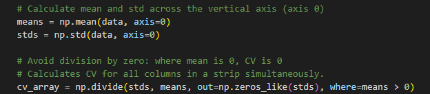
The coefficient of variation is 0 where the rod is smooth. The orange curve on the image above represents [1-CV], allowing us to instead find peaks. The CV array is first smoothed using np.convolve() with a small smoothing kernel, then we compute the 80% percentile using np.percentile(). That’s our green threshold line. The result is that yellow curve that has all the peaks above the threshold using find_peaks() from the SciPy library.

These peaks come and go as the train moves across the tracks. A TemporalRodTracker is used to keep track of the peaks across frames, and merge them with previously recorded peaks using an Intersection over Union (IoU). Each peak is given a score: the highest score is for the peak nearest the center and of the desired width. A peak is considered valid if it has been present for at least 7 frames, and removed if missing for 3 frames. In the example above, the red peak is the best candidate, whereas all the blue ones have either a low score or haven’t been present for at least 7 frames. The values 0.00 (blue) or 1.00 (red) are the current IoU value of each peak compared with the ones from the previous frames.

We also keep track of the global luminosity, in this case the median of the luminance in the region-of-interest. That’s used to detect tunnels: when the train enters a tunnel, all luminance values quickly drop to zero, and since our processing heavily relies on dynamic thresholds using median or percentiles, all the computations become pointless and imprecise.

At the end, once the processor has gone through the entire video, we’re left with a few values for each and single frame: either a valid rod location (that green rectangle on the image above), or a signal we’re in a tunnel and there’s no known rod value. At that point, we can post-process all these invalid frames and use a simple interpolation to fill their rod location.

Detecting the Body of the Rod

Once we have detected the base of the rod, we now want to create a mask that covers the entire rod to be removed. In the original Fuse Lua plugin, this was done by scanning the image line by line, analyzing the contrast left and right of a center. Here the goal is to leverage numpy and OpenCV.

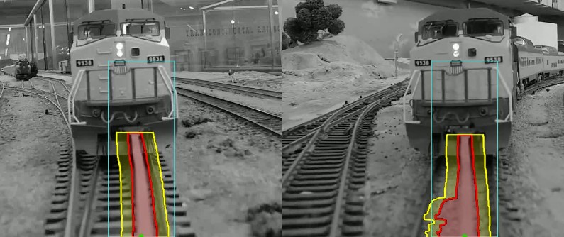
Once we know where the base of the rod is located, we take the bottom center of that rod location. That’s the green dot on the next image. Using the luminance at that spot, combined with the average luminance of the image, we define a threshold to automatically select the pixels that should be the rod in the region of interest:

Red: the opaque rod mask.
Yellow: a smooth gaussian blur on each side for blending.
Green dot: the bottom center of the rod.

As usual, such threshold-based masks can be noisy and non-continuous. To get the desired mask, we apply a variety of OpenCV “morphological transformations”:

• cv2.morphologyEx(cv2.MORPH_OPEN) removes pixel noise using a typical erosion+dilate process.
• cv2.floodFill() is used to keep only the parts of the mask continuous with that starting point (the bottom center of the rod).
• cv2.dilate() is used to expand the mask horizontally.
• cv2.GaussianBlur() is used to create a smooth side edge on both sides of the mask.

Note how the green dot, which represents the bottom center of the rod, is not actually properly centered on the rod. That’s a problem due to the rod tracker using a temporal filter. It tends to lag behind the actual rod movement. This impacts the luminance we’ll be using to compute our threshold.

One problem with this approach is that the luminance often matches the ballast between the ties. To compensate for this, we apply a temporal mask by creating a weighted-AND with the previous frame’s mask. This tends to filter out the part of the mask that matches the ballast as those change from frame to frame, and only the center part of the rod keeps constant from one frame to the next. But it also “erodes” the rod: as it moves left and right, the sides are filtered out by the temporal mask filter. We thus compensate by an horizontal dilate of the mask.

Still, this process results in some false positives. As the example on the right above shows, the mask will still pick up parts of the ties or ballast that has a very close luminance and is long enough to be present over several frames.

Another problem here is that we don’t know where the top of the rod is located, since we don’t track the coupler’s location. We use a heuristic based on the luminance threshold: the top of the rod is darker, thus we stop finding the rod when the luminance goes below our threshold. That results in misses too where a part of the top of the rod is not matched. To compensate for this, we can use some temporal stability: the top of the rod should be somewhat consistent from one frame to the next, so we use a weighted moving average. Still, the approach is problematic. An example is provided below.

Inpainting

“Inpainting” is the process of replacing part of the image by blending it with other parts of the surrounding image. OpenCV has the cv2.inpaint() method to do just that -- it’s very easy to do as all it takes is an input image, and a mask which we just computed, so let’s try it out:

  cv2.INPAINT_NS vs cv2.INPAINT_TELEA

Although very easy to use, these two algorithms are not really suitable for our application. All the examples I’ve seen online use them to fix thin details -- like scratches on an image, or wire removal, and I can see them working adequately for that. It’s fairly clear that the fairly large image mask we provide does not work well for these inpaint algorithms.

The previous Fuse Lua plugin used an inpainting technique which was fairly simple: simply copy pixels left and right from the rod, merging them in the middle. Unfortunately that resulted in some weird artifacts due to the blending of the left and right sides of the rod image. Often, the rod would be closer to the right rail, or the left rail, and thus it picked part of the rail.

I realize that for now, I don’t have a good way to detect if the rod is close to a rail -- I’ve experimented with something like computing a coefficient of variation or using a first derivative of the luminance for each row in order to detect contrast changes, but that has proven quite difficult. So for now, I decided to just encode 3 versions of the Fuse inpainting, yet using numpy operations instead of per-pixel operations.

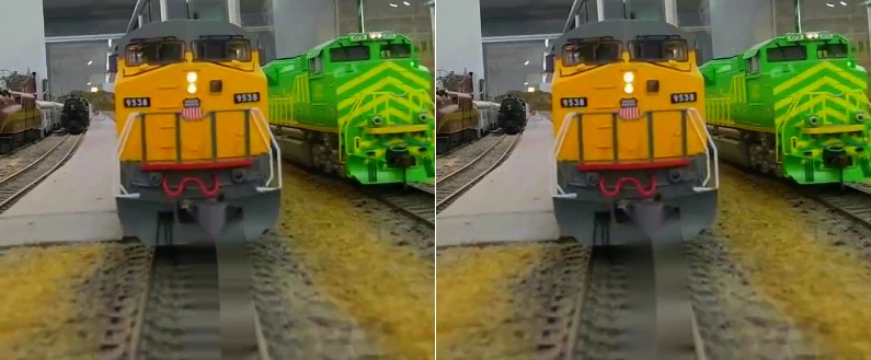
Inpaint left                  Inpaint Mix                  Inpaint Right

In the video shown above, the rod is most of the time on the right side of the image. The “left” algorithm above means to take the image that is to the left of the rod, mirror it, and copy it over the rod. We blend on the opposite part of the rod (the right side) to create a smooth transition.

Similarly, the “right” algorithm mirrors the right part of the rod. That’s fairly visible in the image above on the right: the right rail is mirrored and duplicated in the middle, where the rod used to be.

The “mix” algorithm is exactly what the name implies: it computes both the left and the right versions, and then blends them together. That actually corresponds to what the Fuse Lua code used to do in DaVinci. It often creates these ghost lines because it tends to pick up one rail or the other.

In the new workflow, I simply compute both “left” and “right” inpainted videos, and then pick whichever looks best when editing with DaVinci Resolve.

Limitations and Follow Up

Overall the implementation of this PyRod tool version 1 worked as expected, however the results were not optimal. There were several issues:

• The idea of the temporal filters is very nice on the paper yet… they actually fail to deliver. The rod base detection suffers from lag -- when the train is in a curve, the rod tracker lags several frames behind the actual ideal rod location.
• This in turn means we don’t get the proper bottom center for the rod -- it’s often offset a tiny bit, impacting the actual luminance we use for our threshold. This could be fixed if we were instead using that point to find the one with the best luminance nearby.
• We treat the rod mask as a generic bitmap, totally ignoring the actual geometry of the rod itself. The sides of the rod are always “lines”, even if curved due to perspective. They could be modeled using a polynomial approximation to get rid of the noise generated by the ballast on the left and right of the rod.

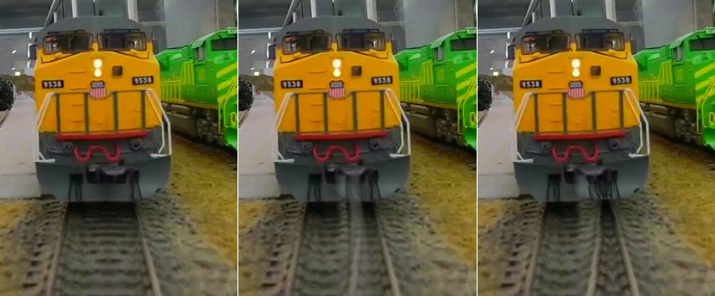
The main issue is the luminance threshold used to detect the rod. This is not a signal as stable as desired, and it results in two kind of misses: the top of the rod is sometimes not matched and keeps being visible, and the width of the rod may not be entirely covered. The latter can be overcome by using a larger horizontal dilate of the mask, but that then impacts the inpaint width negatively.

Left: top of the rod is not properly matched.
Right: width of the rod is not properly matched.

This project can be found on GitHub: https://github.com/alf-labs/rod/tree/main/pyrod1 

Next month, we’ll discuss the version 2 of the tool that compensates for this and generates proper results.

---