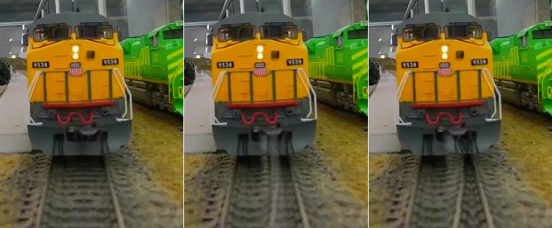
In this article, we’ll discuss the version 2 of the PyRod tool that I use to erase the rod used to attach a camera car to film an HO model train:

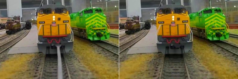
Original image captured by camera               Desired image for the final video

If you haven’t, you may want to read the explanations on PyRod Version 1 here first.

For further details, you can read this blog post that explains the camera car setup that I use to film HO model trains:

The camera car setup.

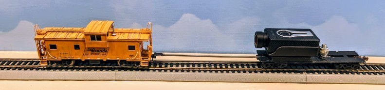
The problem is the 3D-printed rod that attaches the camera car to the train. It’s distracting once seen on the video, and needs to be removed. PyRod is a Python program that does just that.

Version 2 generates proper results like this:

In the previous article, I explained how PyRod Version 1 worked and its shortcomings. So now let’s detail how Version 2 addresses these.

Overview of PyRod 2

The tool is a Python script that processes a source video -- the one captured by the camera. It runs a multi-pass process. Each pass performs one specific action and generates either a video or JSON data for the next pass. The second iteration is structured fairly similarly to the first one. I use the same “engine”, with just a variation on the processors.

GitHub: https://github.com/alf-labs/rod/tree/main/pyrod2 

The structure of the Python project is as follows:

• setup.sh: A wrapper script to create a Python Virtual Environment and install the numpy and opencv-python packages. OpenCV can be quite tricky to install -- it comes with a number of prebuilts that are tightly linked to specific versions of Python depending on whether you run it on Linux or Windows MSYS. Trying to build from scratch is an exercise in frustration that rarely ends well.
• pyrod.py: the main entry point. It decodes command line parameters, loads the input video, invokes one or more “processors”, and writes the output video and json data.
• processor.py: the base class for processors. A processor performs one pass on the video, receiving all the video decoded frames. A processor returns the video to be output, and accumulates whatever data is needed for a later pass. The data can be saved and then reloaded as JSON.
• process_coupler.py: the first pass processor. It runs a tracker that locates the coupler at the top of the rod. Details below.
• process_detector.py: the second pass processor. It determines the outline of the rod.
• process_inpainter.py: the third pass processor. It uses the previously computed coupler location and the rod outline to perform the actual inpainting.

Performance wise, the source is a 4K video, yet we don’t need to process the entirety of the frame every time. To speed up processing, a 1280x720 area is cropped out and processed. Thus all the processors deal with a 1280x720 image at most. Then the generated image is recomposed with the original 4K image to save a 4K video matching the original size and fps.

Each processor has vastly different characteristics yet overall they operate at a speed around 15 to 30 fps rate each on my desktop i5-4400 processor. The overall end-to-end processing speed is around 5 fps though, as it turns out that encoding a 4K mp4 video is quite time consuming.

The Coupler Tracker

Before starting this project, I had already created a DaVinci Fusion plugin that performed the rod removal. This plugin required me to set up a tracker in Fusion to locate the coupler at the top of the rod and track it along the video. That provided the information needed by the plugin to locate the rod below the coupler:

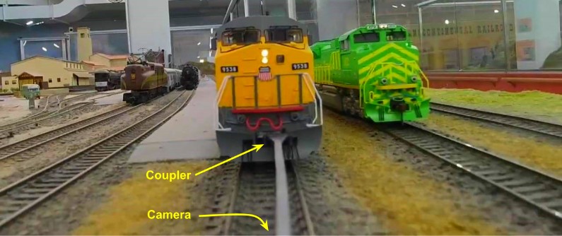
One of the goals of the PyRod Version 1 implementation was to be able skip that coupler tracker as it turned out to be quite a cumbersome task in DaVinci Fusion. The idea was to automatically locate the rod by finding its base -- with the observation that the base of the rod necessarily was in the bottom center of the video and thus should be “easy” to find.

That actually highlighted one of the shortcomings of PyRod Version 1: it turned out that the base of the rod wasn’t trivial to find in a reliable enough way. It moves around when the train runs along a curve, and various tunnels and other places create illumination challenges. The second issue was that the coupler at the top is actually very useful information -- without knowing its location, we cannot reliably figure the height of the rod in the image as it varies while the train bounces around on the track.

Thus in PyRod Version 2, I went back to the notion of tracking that coupler.

It turns out that OpenCV has a neat cv2.matchTemplate() that performs exactly the same kind of template-based tracker as what DaVinci Fusion does:

 

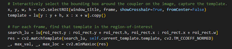
How this works:

• As usual, we first convert our input frame from RGB to L*a*b and extract the luminance channel. All the work is done on the luminance, which provides the best contrast for our search.
• We use cv2.selectROI() once. This displays the frame in a window and the user can draw a bounding box around the coupler area. The template is then saved to the JSON data, to be reused later. Thus we need to do this only once per video, not every time we run the tool.
• For each frame, we compute a region-of-interest where the coupler and the rod are likely to be located. This region is updated dynamically as we progress through the video.
• We run cv2.matchTemplate(). This finds the template within the region of interest using a convolution. The result is a [0..1] map representing the most likely location of the template in the region of interest.
• cv2.minMaxLoc() returns the point in the result map with the highest match. That’s the location of the coupler template in this frame.
• Rinse and repeat for every frame, adjusting the region of interest to somewhat follow the coupler location we found.

The “heatmap” result of the matchTemplate() convolution.
Yellow: The region-of-interest search area.
Green: The matched coupler location.
0.91 is the convolution value at the peak (red spot).
0.28 is the quality score.

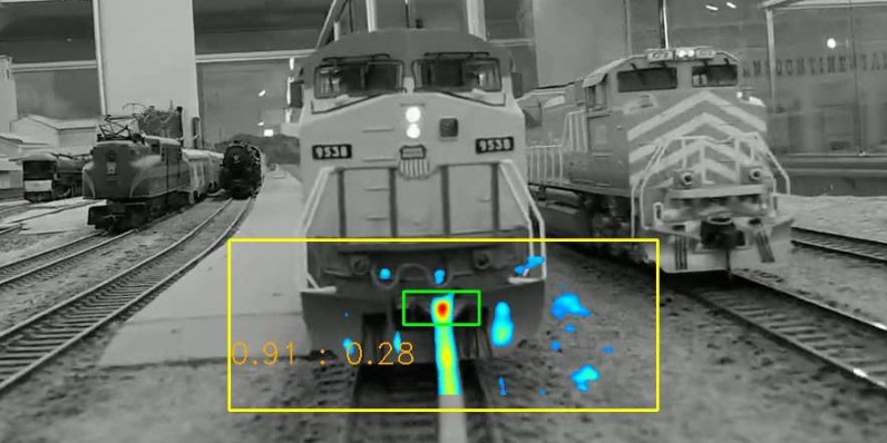
The result of cv2.minMaxLoc() is the location point of the highest template convolution result, as well as the value of that convolution in a [0..1] range. We multiply this with the median of the luminance of the region of interest: this gives us a “quality” score which essentially plummets to zero when the train enters a tunnel. That allows us to ignore fairly dark frames, where the cv2.matchTemplate() fails to give any meaningful result anyway.

The region-of-interest rectangle dynamically moves around to follow the coupler. This has two main purposes: first, we limit our search to a subpart of the image, which makes it fairly fast. Second, the region can only move with some constraints, namely it follows the coupler using a weight-average movement, and its height is constrained to where the rod must end in the image. This prevents the search from “losing its focus”, a problem typical of a tracker in DaVinci Fusion -- sometimes the tracker will latch on some other detail in the image, and once the region of search is no longer overlapping on the desired artifact, it won’t be able to “fix” itself to go back to the real item to be found.

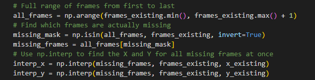
At the end of this pass, we have a list of all possible coupler locations for each frame where the quality was greater than some threshold. We then simply fill the locations for all missing frames using a simple interpolation.

The Rod Detector

The second pass is to detect the outline of the rod.

In PyRod Version 1, we used some kind of flood fill to build a mask using the median of the luminance of the rod at the bottom center point. That proved to be too finicky but more importantly it highlighted the issue that the rod may have inconsistent luminance across its length.

So instead we take a row-by-row approach:

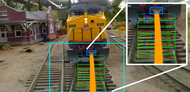
For each row below the coupler tracker, we analyze the luminance of a specific width of that row by finding all locations where the luminance is above the 80% percentile in the row. We then filter these areas using their width and their location -- because we know the ideal width of the rod for a given row, we want one band that has the ideal width and is the closest to the center of the row. This is shown in the control output above: a few selected rows are sampled and displayed; the yellow line is the luminance, the horizontal orange line is the 80% percentile, and the dark blue peaks indicate potential locations above that threshold.

Sometimes, the rod blends with the ballast between the ties. We detect that by computing the min-max contrast for each row. If it’s too low, we simply skip the row as the result would be inaccurate anyway.

For each row, that gives us a potential center and width for the rod. There’s some noise to it, as well as some missing points due to low contrast. To remove the noise, we use numpy's Polynomial.fit to compute a 2nd-degree polynomial approximation of the vertical center line and its width. In the control output above, that polynomial is displayed as the large orange band. It fairly accurately matches the rod.

When we tracked the coupler in the previous pass, we also computed a “quality” score to detect dark areas where tracking was not accurate. We use the same signal here to simply bypass and skip these frames, as they would be too dark to accurately compute the 80% threshold on the luminance. Instead, at the end, we do another quick pass to fill any missing frame data using interpolation.

Inpaint of the Rod

In PyRod Version 1, the second pass was detecting the rod, computing its mask, and performing the inpainting all at the same time. In Version 2, I’ve separated them since the detector phase computes the polynomial outline of the rod and then at the end interpolates it for all the missing frames.

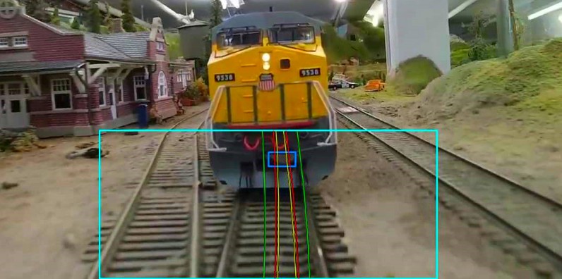
Inpainting uses the same left/right custom-made algorithms I used in Version 1, albeit updated to use the polynomials that define the rod. Here’s an example showing the rod boundaries and the rod inpainted:

Dark blue rectangle is the coupler location.
Yellow curve: opaque center matching the rod.
Red curve: horizontal dilate to cover borders.
Green curve: A smooth blend on each side.

The same 3 possible choices are available for inpainting:

Inpaint left                  Inpaint Mix                  Inpaint Right

Here’s an attempt at explaining the “left” inpaint algorithm:

• The rod boundaries are computed and given by two polynomials: one for the center of the rod, and one for its width.
• For a given row, we compute the rod boundary (yellow lines), and dilate them horizontally (red lines). This accounts for the edges being fuzzy.
• The part between the 2 red lines (left0 → right0) is copied with an opacity of 100%. In the “left” algorithm, we take the part of the row immediately on the left red boundary.
• On the left side, this creates an implicit “smooth” transition since the image is mirrored with itself.
• On the right side, we want to avoid an abrupt transition. The right0→right1 zone also mirrors the pixels from the left side, but this time merged with a progressive opacity blending from 100% down to 0%.

This works well as long as the part on the left of the rod is uniform ballast. It does create artifacts when the rod gets closer to the rails -- either the left rail gets copied to the right, or the right rail gets erased by the pattern. That effect is particularly visible when crossing turnouts or in curves.

In the sample image above, we can see that the “inpaint right” mode duplicates the right rail because it’s too close to the rod.

This described the “left” inpainting method. The “right” one is exactly the same, but swapped left and right.

The “mix” one is, as the name suggests, a mix. It’s however done differently from Version 1: both “A” segments from the right and the left are copied on top of the rod and blended together. Then the progressive opacity blend is performed both on the left and the right. If the rod were perfectly centered with enough sides between the rails, that method would have very good results. Unfortunately, that’s rarely the case and as such it tends to create ghostly artifacts in the middle where the rod used to be.

Inpaint of the Coupler

The coupler is often way too visible in the generated picture, since it results in a fairly light-gray shape on top of the dark engine’s cowl.

PyRod Version 2 adds a simple way to deal with this: In the coupler’s tracked rectangle, we figure the max and median luminance at the base of the coupler. This is used with a cv2.floodFill() to create a mask matching the coupler’s brightest luminance area, and then that area is simply clipped to the median luminance. In other words, we remove highlights. This keeps the coupler’s shape and color intact, yet make it dark enough to match its immediate surroundings, and thus much less noticeable without doing an actual inpainting.

Conclusion and Follow Up

My video workflow so far has been to compute all 3 inpaiting versions and then pick the best one for each segment. In the latest video, the “left” inpainting is used almost everywhere except in two curves where the “right” one had best results. The “mix” one is never used.

Compared to the original DaVinci Resolve plugin that I started with, PyRod Version 2 is a vast improvement. The only input needed is manually selecting the coupler’s boundary once per video, and then saving it as a JSON data file so that I can reuse it. There are a few parameters that I can adjust, such as the rod’s width. However since these are tied to the design of the rod and the camera car, they are going to be consistent for future videos.

One thing I’d like to do is get a better inpaiting that avoids duplicating the rails or erasing them. So far, my attempts at detecting the side rails in the image have not been very successful -- that works in ideal conditions, and spectacularly fails most of the time as the rails are often hard to distinguish from the ballast. It’s easy to guess their location in straight lines, yet hard in curves. Lastly, I’ve been considering some ML approaches for the inpainting, yet so far I have not found any adequate libraries that can run locally on my i5-4400 desktop at reasonable speeds.

This project can be found on GitHub: https://github.com/alf-labs/rod/tree/main/pyrod2 

---